Linear Models Module

To be added.

ZINB-Grad: A Gradient Based Linear Model Outperforming Deep Models

scRNA-seq experiments are powerful, but they suffer from technical noise, dropouts, batch effects, and biases (See this link for more detail).

Many statistical and machine learning methods have been designed to overcome these challenges. In recent years, there has been a shift from traditional statistical models to deep learning models. But are deep models better for scRNA-seq data analysis?

Published literature claimed that deep-learning-based models, such as scVI, outperform conventional models, such as ZINB-WaVE. Here, we used a novel optimization procedure combined with modern machine learning software packages to overcome the scalability and efficiency challenges inherited in traditional tools. We showed that our implementation is more efficient than both conventional models and deep learning models.

We assessed our proposed model, ZINB-Grad, and compared it with scVI and ZINB-WaVE, both developed at the UC Berkeley, using a set of benchmarks, including run-time, goodness-of-fit, imputation error, clustering accuracy, and batch correction.

Our development shows that a conventional model optimized with the proper techniques and implemented using the right tools can outperform state-of-the-art deep models. It can generalize better for unseen data; it is more interpretable, and not surprisingly, it uses extremely fewer resources compared to deep models.

Table of Contents

• ZINB-Grad: A Gradient Based Linear Model Outperforming Deep Models

  • Table of Contents

  • Project Organization

  • ZINB-WaVE

    • ZINB-WaVE Bottleneck

  • ZINB-Grad

  • Results And Model Evaluation

    • Run-time

    • Generalization

    • Imputation Evaluation

    • Clustering

    • Batch Effect Correction

  • Conclusion

ZINB-WaVE

ZINB-WaVE is a generalized linear mixed model (GLMM) which captures the technical variability through two known random variables and maps the data onto a biologically meaningful low-dimensional representation through a linear transformation. ZINB-WaVE extracts low-dimensional representation from the data by considering dropouts, over-dispersion, batch effects, and the count nature of the data.

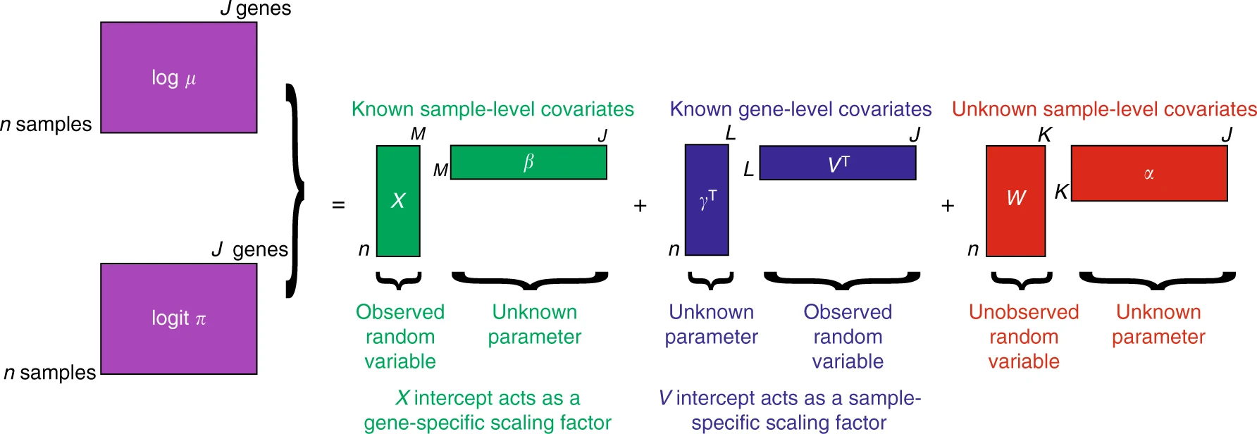
In the above schematic graph, $X$ and $V$ are known sample-level and gene-level covariates, respectively. $X$ can model wanted or unwanted variations. For instance, $X$ can be used to correct batch effects, and $V$ can model gene length or GC-content. This is how ZINB-WaVE performs normalization and batch effect correction all in one step.

$W$ and $\alpha$ are the unknown matrices that are used for dimension reduction. Columns of $W$ are essentially the latent space of ZINB-WaVE, and $\alpha$ is its corresponding matrix of regression parameters. The $O$ parameters are the known offsets for $\pi$ and $\mu$. For more details, please refer to ZINB-WaVE.

ZINB-WaVE Bottleneck

The bottleneck of the ZINB-WaVE is in its estimation process, which includes several iterative procedures, such as ridge regression and logistic regression. It also contains SVD decompositions of big matrices (for large sample sizes) and the BFGS quasi-Newton method. Not surprisingly, the optimization procedure requires heavy computations and high-memory storage. Therefore, the ZINB-WaVE is doomed to be scalable to only a few thousand cells, and nowadays, applications require millions of samples to be efficiently analyzed.

However, this limitation does not imply that the traditional linear models are suboptimal compared to deep learning-based models. Indeed, we will show that, by switching the optimization procedure from the conventional analytic way to a modern method, ZINB-WaVE is scalable to millions of cells and even more efficient and productive than its deep learning descendent, such as scVI.

ZINB-Grad

Supported by most modern machine learning packages (e.g., Pytorch and Tensorflow), gradient descent and its variants are used to optimize deep neural networks and are among the most popular algorithms for optimization. By updating the parameters in the opposite direction of the objective function’s gradient, gradient descent finds local optimum values of the model’s parameters to minimize the objective function regardless of how complicated is the model.

However, a neglected fact is that gradient descent may also be applied to “simpler” linear models when appropriate. Towards this line, we developed a gradient descent-based stochastic optimization process for the ZINB-WaVE to overcome the scalability and efficiency challenges inherited in its optimization procedure. We combined the new optimization method with modern statistical and machine learning libraries, which resulted in the ZINB-Grad, a gradient-based ZINB GLMM with GPU acceleration, high-performance scalability, and memory-efficient estimation.

Results And Model Evaluation

We evaluated ZINB-Grad using a set of benchmarking data sets and a range of technical and biological tests. We used three benchmarking datasets, namely, CORTEX, RETINA, and BRAIN.

Run-time

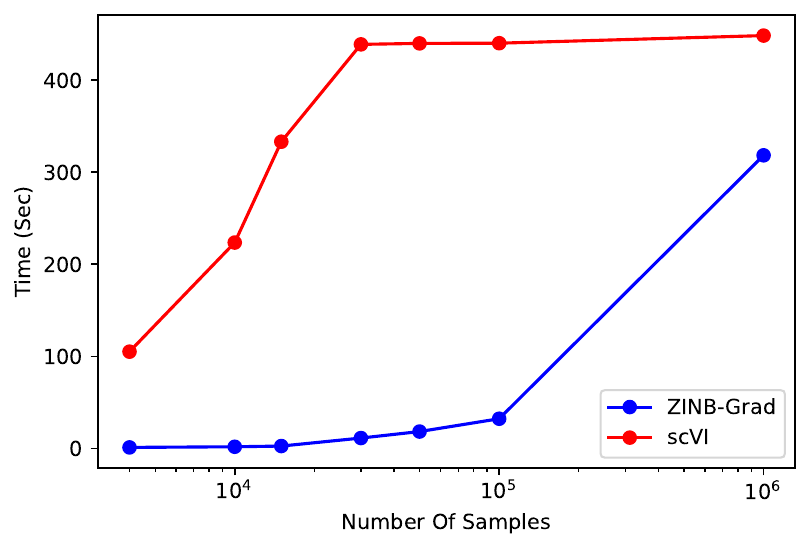
Since Lopez et al. have clearly shown that scVI is significantly faster than ZINB-WaVE for comparable data set sizes, and for > 30,000 samples, ZINB-WaVE cannot scale, we did not test ZINB-WaVE’s run-time.

Our analyses showed that ZINB-Grad run-time is exceedingly lower than the scVI for any data size (the following plot) due to the simplicity of the model. All scVI and ZINB-Grad tests were performed using a computer equipped with a V100 GPU and 32 GB of system memory for GPU acceleration.

Generalization

We examined the ZINB-WaVE goodness-of-fit for the train data as a reference for our model (ZINB-WaVE cannot scale to > 30,000 sample). ZINB-Grad has the same (or even better) negative log-likelihood compared to ZINB-WaVE for various data sizes (below figure). Therefore, our optimization procedure will get a minimum of comparable quality to ZINB-WaVE’s estimation process. The train negative log-likelihood for ZINB-Grad is the same or better compared to scVI.

Moreover, the negative log-likelihood of the validation set for ZINB-Grad is better than scVI in any data sizes (following figure), showing that our linear model generalizes (extrapolates) better than a deep model even for large sample sizes.

Imputation Evaluation

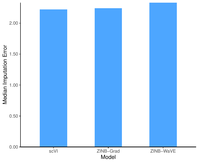
We corrupted the data by randomly selecting 10% of the non-zero entries and altering them to zero. Then, we used the median of the ${\mathbb L}_1$ distance between the original and imputed values of the altered data set as the accuracy for data imputation.

We corrupted the CORTEX data set, and then, we estimated the parameters of the models using the corrupted data set. Finally, we compared the original data set (before corruption) with the imputed data from the models trained with the corrupted data set using the median ${\mathbb L}_1$ distance. The following figure shows the performance of the three models in terms of imputation error. ZINB-Grad performance is comparable with scVI and is better than ZINB-WaVE.

Clustering

We performed clustering on the latent space with 10 dimensions for scVI, ZINB-WaVE, and ZINB-Grad using K-means. We calculated the Normalized Mutual Information (NMI) and Adjusted Rand Index (ARI) between the gold standard labels of the CORTEX data set and labels obtained from K-means, along with Average Silhouette Width (ASW) to assess the clustering performance of the ZINB-Grad compared to scVI and ZINB-WaVE (below figure). For all scores, NMI, ARI, and ASW, the higher is better.

ZINB-Grad and ZINB-WaVE scores are close, and the clustering scores show that ZINB-Grad performed slightly better than scVI.

Batch Effect Correction

We evaluated the accountability for technical variability by assessing batch entropy of mixing and visualizing the latent space in the RETINA data set containing two batches. We performed two experiments to visualize the effect of batch correction. In one experiment, we corrected the batch effect; in the other one, we did not.

• The following figure show the latent space of the ZINB-Grad when batch annotations are not considered (Blue dots are Batch 1 and Green dots are Batch 2):

• The different clusters (cell types) when batch annotations are not modeled:

These graphs show clearly that without performing batch correction, the technical variability will cause the cells in the same cluster (cell population) to construct different clusters, which will be misleading in the downstream analysis.

• The following figure show the latent space of the ZINB-Grad when batch annotations are considered (Blue dots are Batch 1 and Green dots are Batch 2):

• The different clusters (cell types) when batch annotations are modeled:

These graphs show that after considering batch annotations, ZINB-Grad accounts for the technical variability and results in a biologically meaningful latent space.

We used the entropy of batch mixing to measure the batch effect correction. We randomly selected 100 cells from batches and found 50 nearest neighbors of each randomly chosen cell to calculate the average regional Shanon entropy of all 100 cells. The procedure is repeated for 100 iterations, and the average of the iterations is considered as the batch mixing score. We could not use ZINB-WaVE for the RETINA data set as it was too large for ZINB-WaVE to handle. The batch mixing scores for scVI and ZINB-Grad are 0.64 and 0.54, respectively.

Conclusion

We showed that our implementation is more efficient than both conventional models and deep learning models. Moreover, our model is scalable to millions of samples and has performance comparable with deep models in terms of accuracy. As the devil is in the implementation details, the supremacy of deep models may not be due to their sophisticated deep architecture. Instead, the source of effectiveness is merely the optimization procedure built-in to deep models implementations, which could also be adopted by many traditional models.